NBA Game Excitement Index
15 Feb 2021On 2021-01-30, the Chicago Bulls played the Portland Trail Blazers in an exciting regular season game. Unfortunately for Bulls fans, the Trail Blazers won the game with an epic comeback to erase a 5 point deficit capped by two clutch three point shots in the final 8.9 seconds by Damian Lillard.
After watching this game, I thought:
- Was this the most ‘exciting’ game the Bulls have played this year?
- How does this stack up relative to other Bulls games in terms of ‘excitement’?
Research
In order to answer these questions we need to define what it means for a game to be exciting. One mearsure of excitement that I found interesting was documented by Luke Benz on the Yale Sports Analytics Site. Although the formula as specified is for a college game it is easily modified for NBA games.

In words, this metric is measuring how much the Home teams win probability changes over the course of the game. Games with many lead changes, or dramatic changes in Win Probabilities, should naturally result in an exciting game. Additionally, we want to normalize for the length of the game, so we normalize to a standard game length.
Given the formula above, we need to obtain Win Probabilities in order to calculate this ‘Game Excitment Index’.
Data
On github there is a project called nba_api that makes it easy to access statistics directly from the NBA website. Thankfully Win Probabilities are part of the data that is provided.
Using the nba_api one can access the Win Probability data using the following:
Where GAME_ID is just a unique game identifier that can be accessed via other nba_api calls.
The above code block retrieves the win probability data as a Pandas dataframe. The Win Probability is reported for each second of the game starting from the opening tip through the end of the game, including any overtime periods.
The key columns in the Win Probability data required to calculate the Game Excitement Index are:
- GAME_ID - The unique game identifier
- HOME_PCT - The home team win probability as of a time in the game
- VISITOR_PCT - The visiting team win probability as of a time in the game
- PERIOD - The period of the game. Values 1 through 4 indicate regulation time and any value greater than 4 is for an overtime period
- REMAINING_SECONDS - The remaining seconds in the current period
An example table for the Win Probability is the following:
| GAME_ID | HOME_PCT | VISITOR_PCT | PERIOD | SECONDS_REMAINING | |
|---|---|---|---|---|---|
| 0 | 0021701024 | 0.58808 | 0.41192 | 1 | 720 |
| 1 | 0021701024 | 0.61352 | 0.38648 | 1 | 720 |
| 2 | 0021701024 | 0.6135 | 0.3865 | 1 | 719 |
| 3 | 0021701024 | 0.61348 | 0.38652 | 1 | 718 |
| 4 | 0021701024 | 0.61346 | 0.38654 | 1 | 717 |
Now that we have the data, let’s calculate our Game Excitement Index and see how the game in question stacks up against other games
Analysis
With the Win Probability data retrieved, we can calculate the Game Excitement Index via the following formula:
According to the metric, the Chicago Bulls vs Portland Trail Blazers game on 2021-01-31 scored 10.5 on the Game Excitement Index.
Before we jump in to see how this game compares to other games the Bulls have played, we can visualize the Win Probability across the entire game.
The following plot has three subplots across the duration of the game:
- Subplot 1 - Home and Visiting Team Win Probabilities
- Subplot 2 - Win Probability Difference or Spread across the game (Home Team Probability - Visiting Win Probability)
- Subplot 3 - Home Team Probability Difference (Home Team Probability at T - Home Team Probability at T-1)
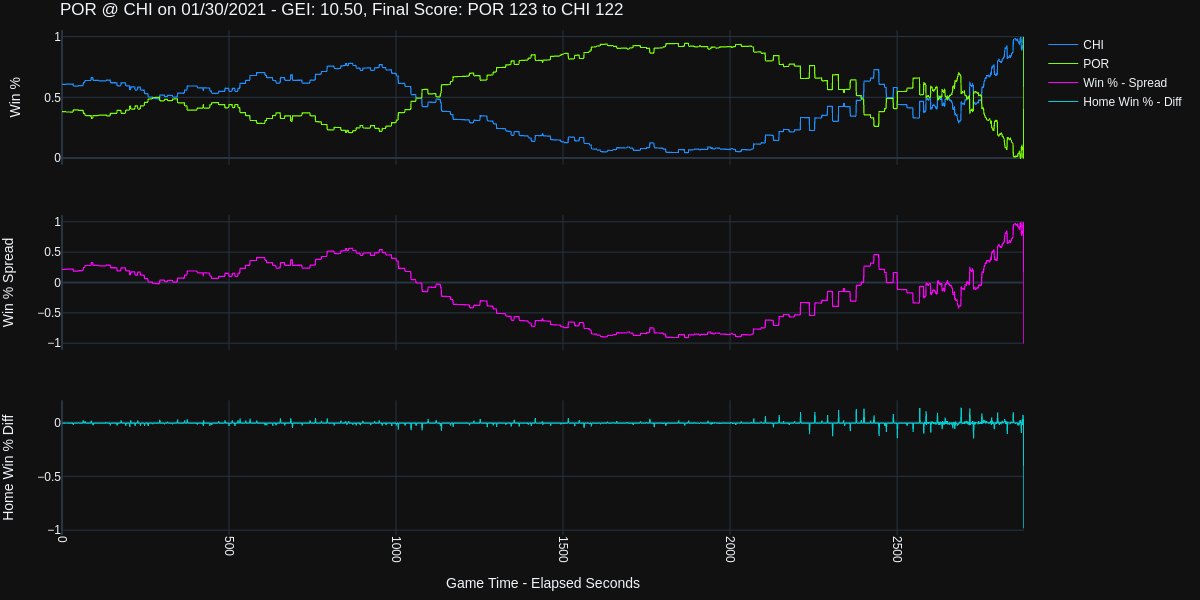
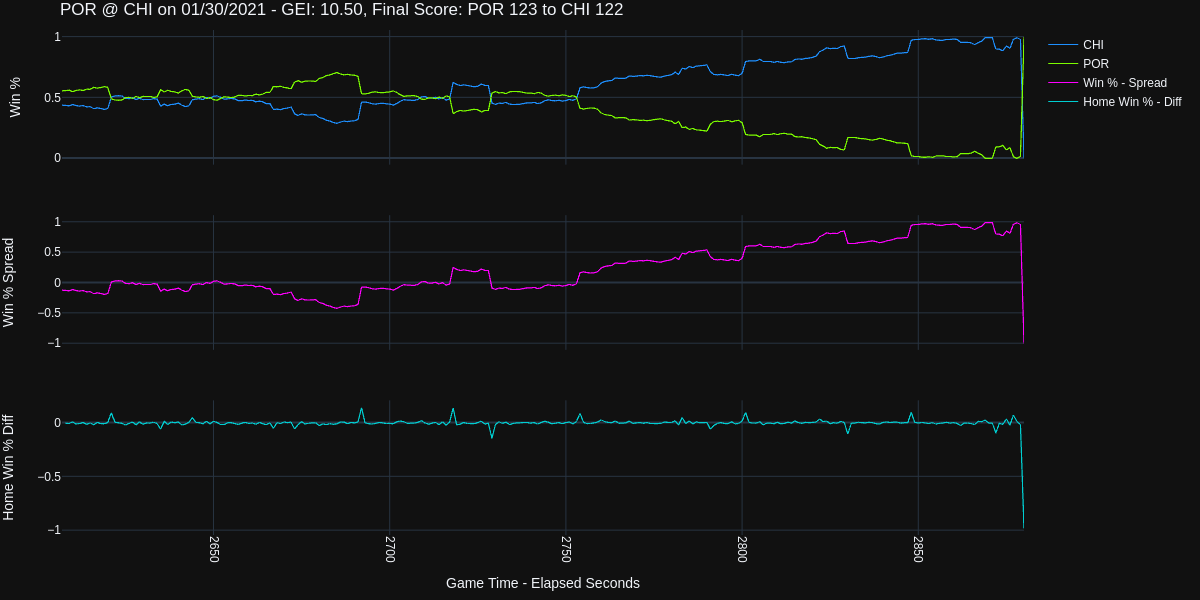
If you zoom into the last 120 seconds of the game, you can see how the Chicago had a Win Probability of close to 100% just prior to losing the game.
According to our metric, here are the most exciting Chicago Bulls games so far this season (2020-12-23 to 2021-02-15)
| game_id | game_date | matchup | wl | game_excitement_index | |
|---|---|---|---|---|---|
| 0 | 0022000063 | 2020-12-31 | CHI @ WAS | W | 12.0052 |
| 1 | 0022000038 | 2020-12-27 | CHI vs. GSW | L | 11.4711 |
| 2 | 0022000142 | 2021-01-10 | CHI @ LAC | L | 11.3359 |
| 3 | 0022000298 | 2021-01-30 | CHI vs. POR | L | 10.5012 |
| 4 | 0022000117 | 2021-01-06 | CHI @ SAC | L | 10.0578 |
It’s a bit surprising that the Portland game is only the 4th most exciting game so far this season. So what happened during the most exciting game? Let’s take a look
This game had lots of back and forth lead changes and an exciting finish with the Bulls taking the victory.
Now how does this game stack up to other games since 2015-01-01. Here are the top 10 games
| game_id | game_date | matchup | wl | game_excitement_index | |
|---|---|---|---|---|---|
| 0 | 0021700065 | 2017-10-26 | CHI vs. ATL | W | 18.1496 |
| 1 | 0021700444 | 2017-12-18 | CHI vs. PHI | W | 15.631 |
| 2 | 0021700466 | 2017-12-21 | CHI @ CLE | L | 15.1372 |
| 3 | 0021701024 | 2018-03-15 | CHI @ MEM | W | 12.6051 |
| 4 | 0022000063 | 2020-12-31 | CHI @ WAS | W | 12.0052 |
| 5 | 0021800970 | 2019-03-06 | CHI vs. PHI | W | 11.9672 |
| 6 | 0021800875 | 2019-02-22 | CHI @ ORL | W | 11.8057 |
| 7 | 0021700537 | 2017-12-31 | CHI @ WAS | L | 11.7761 |
| 8 | 0021800310 | 2018-11-28 | CHI @ MIL | L | 11.7006 |
| 9 | 0021700222 | 2017-11-17 | CHI vs. CHA | W | 11.6912 |
| 10 | 0011500103 | 2015-10-23 | CHI vs. DAL | W | 11.6396 |
| 36 | 0022000298 | 2021-01-30 | CHI vs. POR | L | 10.5012 |
It turns out that the Portland game only ranks 36th in terms of excitment! Or Does It?
Data Issues
Any time you work with data you have to expect some data errors or issues, and the data from the NBA is no different. Let’s take a look at the most exciting game according to our metric
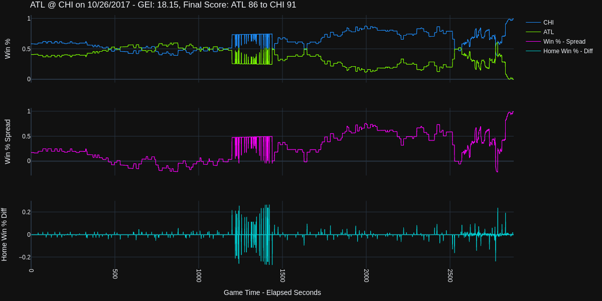
You can see in the above plot that the Win Probability data is strange near the middle of the game. These fluctations have a huge impact on our metric as we are calculating the total change in Win Probability over the length of the game. Small frequent fluctations can have a big impact on this metric.
Unfortunately, a number of games have this issue and it is difficult to identify these issues programatically.
So what was the most exciting game?
The game between Chicago and Mempis on 2018-03-15 scores 12.61 on the Game Excitement Index.
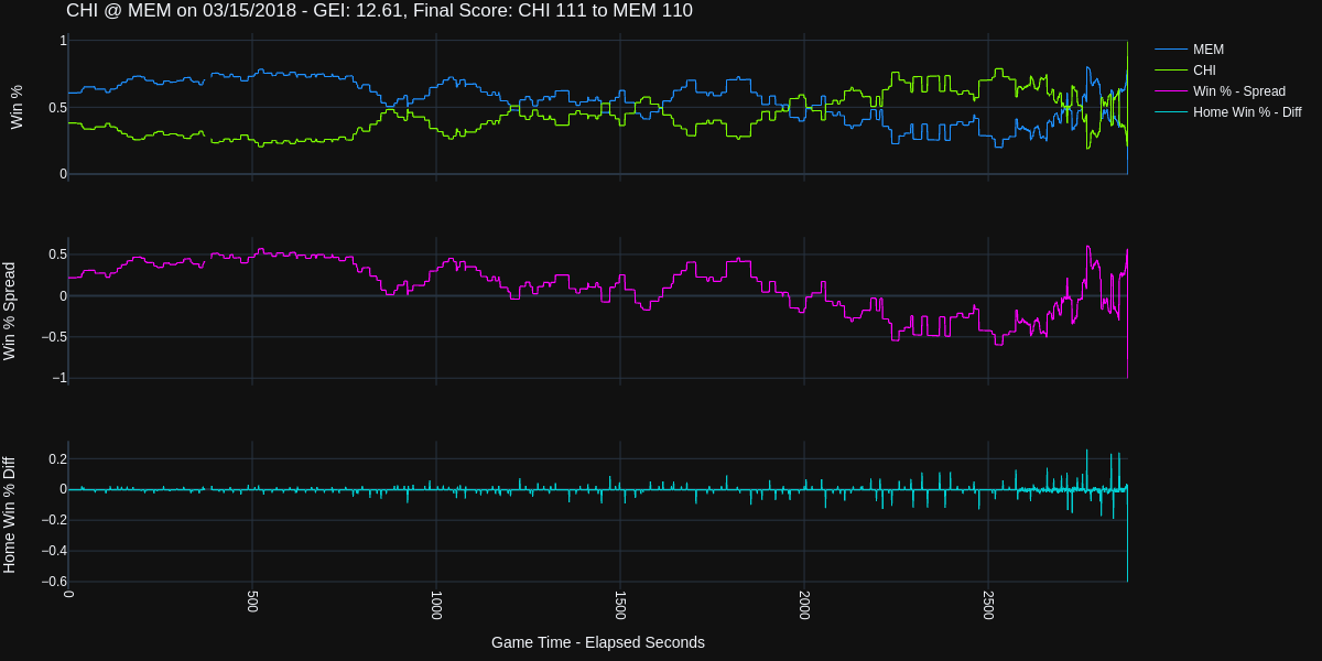
And here is the recap of the game highlights, the ending of this game is incredible!